1.population

data1 = {101654, 103008, 104357, 105851, 109300, 111026, 112704, 
   114333, 115823, 117171, 118517, 119850, 121121, 122389, 123626, 
   124810};
data = Table[{1982 + (i - 1), data1[[i]]}, {i, 1, 16}];

//exponential model
lnm = NonlinearModelFit[data, data1[[1]]*Exp[a*(x - 1982)], a, x, 
   Method -> "NMinimize"];

<!-- more -->

//logistic model
lnm1 = NonlinearModelFit[data, 
  a/(1 + (a/data1[[1]] - 1)*Exp[-b*(x - 1982)]), {a, b}, x, 
  Method -> "NMinimize"]


//plot two models
  Show[ListPlot[data], Plot[lnm[x], {x, 1982, 2000}]]
Show[ListPlot[data], Plot[lnm1[x], {x, 1982, 2000}]]


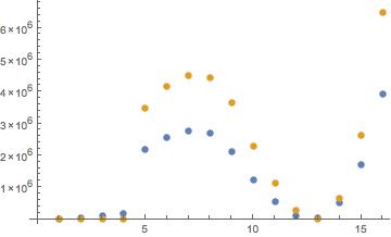
//illustrate the resid plot

ListPlot[{(lnm /@ data1 - data2)^2, (lnm1 /@ data1 - data2)^2}, 
 PlotLegends -> Automatic]

 //make the prediction

 lnm[2015]
lnm1[2015]

Take care of the method in case its invalidability.

method should be set “NMinimize“ to find the overall solution.

exponential model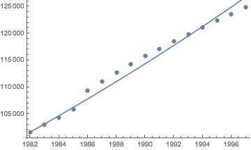

logistic model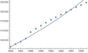

resid plot of two models.

orange represents model1, while blue represents model2

Take care of the method in case its invalidability.

method should be set “NMinimize” to find the overall solution.

3.wolf and sheep

//solution to diffrential equation should be obtrained from N methods. 

sl = NDSolve[{x'[t] == 
     2*(-60 - x[t])/Sqrt[(-60 - x[t])^2 + (t - y[t])^2], 
    y'[t] == (t - y[t])/Sqrt[(-60 - x[t])^2 + (t - y[t])^2], 
    x[0] == 0, y[0] == 0}, {x[t], y[t]}, {t, 0, 60}];
ParametricPlot[Evaluate[{x[t], y[t]} /. sl], {t, 0, 60}];
Show[%, ParametricPlot[{-60, t}, {t, 0, 60}]]

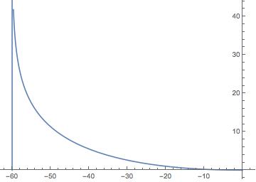
it’s easy for us to discover that wolf was not fast enough to caught the sheep.

4.Integration

//calc and output the numeric answer

Integrate[1/Sqrt[2*Pi]*Exp[-x^2/2], {x, 0, 1}]//N

5.Optimization

//local minimum

FindMinimum[3*x^2 + 10*y^2 + 3*x*y - 3*x + 2*y, {{x, 0}, {y, 0}}]

//minimize(overall optimize)

//In Lingo, x, y are automatically constrained to be big than 0, thus triggerring our @free(x) @free(y) steps .

Minimize[3*x^2 + 10*y^2 + 3*x*y - 3*x + 2*y, {x, y}]

differences between minimum and minimize should be given enough attention

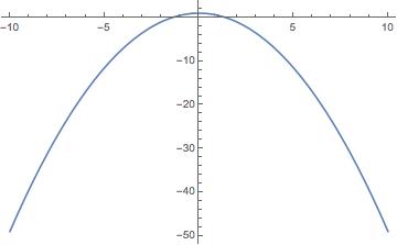
6. Diffrential equation

ans = NDSolve[{y''[t] - 7*(1 - y[t]^2)*y'[t] + y[t] == 0, y[0] == 1, 
    y'[0] == 0}, y[t], t];
Plot[Evaluate[y[t] /. ans], {t, -10, 10}]

it’s necessary to use N method.

And the plot is clear